 Deutsch Deutsch |
Parabolic-dish scooter |
|
1.0 Introduction 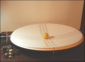
The stalk of a grain plant, which is blown and turned away by the wind, does not bend over because it retreats elastically and, when the wind subsides, it causes oscillations.
Did nature accidentally design this way or is there a principle behind it that is not recognizable at first glance?
We encounter vibrations at many places in daily life. Most people know from the fair the little devils that swing up and down on spiral springs. If you observe closely, you will see that the water surface, which was crushed by a stone's throw, shoots above its normal height. On all musical instruments, barely visible components vibrate, which stimulate the air to sound waves and create the auditory impression in our ears. High-rise buildings are equipped with an elastic steel skeleton so that they can give way like the grain plant during storms or earthquakes. In the watches, balance, pendulum or an oscillating quartz work for an exact time, the driving comfort in the vehicle is increased by oscillating damped suspension. Even molecules, the atoms in a crystal lattice and even the atomic nuclei and their elementary particles carry out vibrations and thus store energy.
The principle of oscillation is always the same: elastic objects that are brought out of equilibrium by an external force vibrate when they react to the external excitation with a backward, location-dependent force.
Backward means that the force exerted by the object acts opposite to the direction of the stimulating force. Location-dependent means that as further the object is deflected from its equilibrium, as greater the reaction force is.
With the Parabolic-dish scooter you can experimentally measure different physical quantities that determine a vibration. In this experimental setup you will learn a lot about the concept of vibration. And once you understand the general principle, you can apply it to many different areas of physics.
You will learn important things about measurement technology while experimenting. The sensible execution of the experiments is a prerequisite for good results.
With every measurement, measurement inaccuracies occur that you cannot avoid.
For example, if you let several people measure the height of a tabletop, you get different results (77.3 cm, 77.2 cm, 77.7 cm, 77.55 cm, 76.9 cm...). The measured values scatter around a certain value, the average value, which here is 77.33 cm. The range in which the measurement results occure, here ± 0.4 cm, is called measurement uncertainty. If you can specify the range of measurement uncertainty, you are able to make a statement about the accuracy of your measurement.
certainly, one goal is to make this value as small as possible.
2.0 Experimental setup The experimental setup consists of a parabolic-antenna dish with axis lengths of 72 cm and 83 cm. On a board, the bowl is stored on four height-adjustable tips. In the parabolic dish you can run different balls and cylinders back and forth. If you start the "scooters" at the edge, they perform vibrations and remain after some time in the lowest point of the bowl. For the experiments you need different objects from the following table. Please check at the beginning of your experiments if everything is there.
A vibration is a periodic movement. In this example, a rolling object performs a vibration in the parabolic dish. There is a fixed physical quantity for this movement:
The oscillation duration, which describes the movement and depends on the structure of the bowl and the properties of the materials used. The oscillation duration is the time it takes for the deflected scooter to return to the same state. These can be any places i, but also the maximum
end positions in the bowl.
The number of oscillations that the scooter performs in one second is called frequency and is measured in units [1/s] or Hertz [Hz]. It can be calculated as a reciprocal from the oscillation duration. The frequency of the satellite roller can also be less than 1 Hz. If the system is left to itself, it usually oscillates at a very characteristic frequency, such as a pendulum. This frequency is called natural frequency. The largest deflection of an oscillation is called amplitude.
The rolling speed is not constant in vibration and is affected by friction between the roller and the bowl surface. The friction causes the amplitude to decrease over time. After some time, the state of equilibrium, namely the resting position, usually at the lowest point of the bowl, occurs.
4.0 First observations 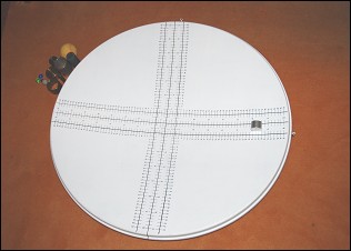
It is best to do a trial phase first. Bring the bowl with the adjusting screws and the spirit level into a horizontal position. You have to make sure that the screws do not protrude from the board below. The maximum adjustment travel is determined by the board thickness and the height of the mounting blocks. Now let a scooter of each type roll from certain heights (deflection) or from the edge of the bowl into the rest position. Limit yourself to the 2 axes. How many vibrations can you observe on which scooter? How long does a vibration last? Where do the scooters stop? Is the magnitude of the deflection related to the oscillation duration or the number of oscillations?
You now have an idea of what happens to the scooters. But now your experiment should be more precise. Good scientists first describe their experimental setup and then what and how they have measured. An important scientific tenet is the verifiability of your results by others. So you should now be able to generate real measured values and also say how good they are.
5.0 General information Quantitative measurements make experiments comparable. This also makes it possible to check predictions from theory. With every measurement, however, measurement inaccuracies arise, which of course have nothing to do with incorrect work. Only by specifying the size of these inaccuracies the quality of the measured values can be assessed.
5.1 The following measurement inaccuracies may occur:
5.2 Possibilities for error limitation and error estimation:
It was already mentioned in the introduction: The oscillation duration is the time that the deflected scooter needs to meet the same place again. Depending on the starting location, these can be any places in the bowl. The axles are of course predestined.
6.1 Vibration duration tasks 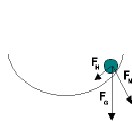
Since these measurements are time-critical, it makes sense that you think about the process before the measurement.
Which physical quantities are measured?
What range of values can they take?
What preparations are important before the measurement?
How are the tasks distributed?
How should the measured value table be created?
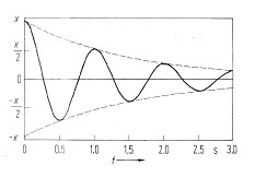
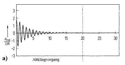
During the first measurements on the parabolic dish, you noticed that the amplitude of the oscillation decreases over time. This oscillation is also called damped oscillation. In the adjacent figure (from literature) you can see an example of how the amplitude of a scooter vibration decreases with time, which was initially deflected by the value x. The reason for the amplitude decrease of the oscillation is the friction of the roller on the bowl surface. Due to friction, vibrational energy is lost, the amplitude of the oscillation is dampened. Depending on the degree of attenuation, three cases can be distinguished:
8.0.1 A harmonic oscillation occurs when - as already explained in the introduction - location-dependent, driving forces are present in a system. In the satellite scooter, the downhill
force, a component of gravity, is involved as a driving force. After starting the scooter at the edge of the parabolic-antenna dish (excitation of the oscillation), the positional energy (potential energy) of the scooter is converted several times into kinetic energy.
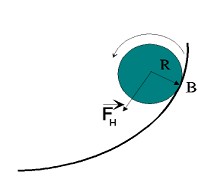
The potential energy follows from the potential function, which you have already determined except for a constant factor (weight force of the rolling equipment) when measuring the bowl surface. From a physical point of view, a potential is a rule from which energy values can be calculated. If you move an object on the key surface between two points of different height (different potential), you must either move it up and do work, or move it down, freeing up work. This work is equal to the potential energy that can also set the scooter in motion if you let it roll freely. The downhill force generates a rotational movement via the lever arm center of gravity - contact point (radius R) a rotary movement. The scooter rotates around its center of gravity, which moves at a distance R above the bowl surface to its lowest point. The rotation can be understood as kinetic energy of the scooter. Analogous to the inertia of a linear motion, the moment of inertia acts in the rotational motion of a body Θ.
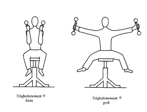
If you own a swivel chair, you can perform a simple experiment to experience the effect of the moment of inertia. Get on a swivel chair, stretch out your arms and legs to get some momentum and rotate yourself (right picture). Then you pull your arms and legs close to your body (left picture). What do you observe? To repeat, you can stretch your arms and legs again.
The moment of inertia is a quantity that takes into account the distribution of mass with respect to its axis of rotation (outstretched, applied arms or legs). To determine the moment of inertia, each mass particle is weighted with the square of the distance from its axis of rotation. If one piece of mass is considered at a distance R1 and another piece of the same size at a distance of 2 * R1 from its axis of rotation, the latter mass has 4 times the moment of inertia. The greater the moment of inertia of a body, i.e. as further away its mass is from its axis of rotation as harder it is to set a body into rotation. If two bodies of the same mass but with different moment of inertia have the same rotational energy, the body rotates more slowly around its axis of rotation with a greater moment of inertia.
The third energy component is the loss energy. If the ball or cylinder rolls over the bowl surface, part of its energy is converted into thermal energy at each oscillation at the support point with each oscillation. This is released into the environment and is lost to the system. The loss is reflected in the amplitude decrease that you have already observed. The ratio of stored energy to loss energy is called quality, Q of the vibrating system.
8.1.0 Tasks relating to the different forms of energy of scooter vibration
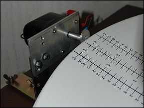
9.0.1 The parabolic dish is mounted on two tips on its longitudinal axis and is driven on the transverse axis on one side by the motor and the eccentric wheel, which converts a rotary movement into a linear movement. A preloaded spring on the opposite side ensures that the bowl always rests against the eccentric wheel. The number of revolutions of the motor can be varied by changing the motor voltage within a sufficient range.
With this arrangement, the parabolic dish can be periodically moved up and down around an axis and the vibration of the rolling equipment can be maintained over a longer period of time. The parabolic dish, which can be tilted in one direction, and the cylinders or spheres rolling in it in the same direction form two oscillating systems, each of which can move with different frequencies or oscillation durations.
According to the superposition principle, these two oscillations overlap, the deflections add up at any time. If you start the scooter at any point of the bowl, it oscillates in its natural frequency, which experiences an amplitude decrease due to the damping. When all the vibration energy is used, the rolling device remains at the lowest point of the parabolic dish (decay process: Fig. a).
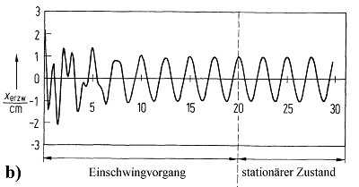
9.0.2 If the drive is switched on in the meantime, the natural oscillation of the scooter overlaps with the excitation by the motor and the scooter performs complicated forms of movement, which are also referred to as the transient process of a forced oscillation (see Fig. b).
9.0.3 If the initial energy of the scooter is dampened away and the periodic drive continues to work uniformly, a stationary behavior occurs (right section in Fig. b).
9.0.4 Whenever the amplitude, phase or frequency of one of the oscillating systems changes, these transient or decay processes occur; if you wait a while afterwards, you have a stationary behavior again.
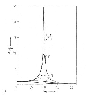
  9.0.5 If the speed of the motor is increased from low to higher values, the scooter oscillates stationary after the corresponding waiting time with an amplitude dependent on the excitation. If the natural frequency of the bowl-roller system is reached, the amplitude assumes a maximum.
9.0.6 This is referred to as resonance.
The lower the attenuation or the greater the quality Q of the system, the higher and the narrower the amplitude curve as a function of the excitation frequency (see Fig. c; resonance curve).
9.0.7 If the excitation frequency is significantly higher than the natural frequency of the scooter, then the amplitude drops again.
 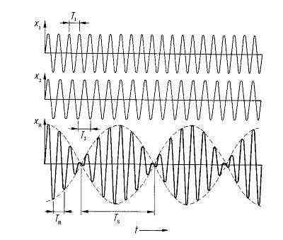 9.0.8 In addition to resonance, there is another special stationary state: beating. Beating occurs in the event that the frequency difference between the excitation and the rolling movement is small and the quality Q of the system is particularly high.
9.0.9 In the adjacent figure, two oscillations are superimposed with the ratio T1/T2 = 7/6.
The result is an oscillation whose amplitude is modulated with the oscillation duration. As smaller the distance between excitation frequency and natural frequency, as greater the oscillation duration TS of the beat is. At the same time, the enveloped oscillation duration TR of the scooter vibration changes proportionally to the reciprocal of the sum of excitation and natural frequency.
10.1 Tasks for excited scooter vibration
|
|
| Copyright by Hans Joachim Ilgen seit 1950 | |